Birth-and-death Processes

BirDePy is built for analyzing general birth-and-death processes. These continuous-time Markov chains (CTMCs) are widely used to study how the number of individuals in a population changes over time. Let $Z(t)$ denote the size of a population at time $t\ge0$; the process $Z\equiv (Z(t),\,t\ge0)$ evolves on the state space $\mathcal S = (0,1,\dots,N)$, where $N$ may be infinite. We assume that the evolution of such a process is fully described by non-negative real-valued functions $\lambda_z(\boldsymbol\theta) : \mathcal S \to \mathbb R_+$ and $\mu_z(\boldsymbol\theta) : \mathcal S \to \mathbb R_+$ of the current state $z$; these functions are known as the population ‘birth-rate’ and ‘death-rate’, respectively. The model has a finite number of real parameters recorded in the vector $\boldsymbol\theta$. When $Z(t)=z$, the time until the process transitions to another state is exponentially distributed with mean $(\lambda_z(\boldsymbol\theta)+\mu_z(\boldsymbol\theta))^{-1}$ (where we define $1/0=\infty$). At a transition time from state $z$, the process jumps to state $z+1$ with probability $\lambda_z(\boldsymbol\theta)/(\lambda_z(\boldsymbol\theta)+\mu_z(\boldsymbol\theta))$, or to state $z-1$ with probability $\mu_z(\boldsymbol\theta)/(\lambda_z(\boldsymbol\theta)+\mu_z(\boldsymbol\theta))$.

As summarized below, we consider selected birth-and-death models of three types: (i) some variants of the linear BDP, (ii) some PSDBDPs, and (iii) some queueing models.

Transition rates and parameters for $z \geq 0$. Any rates which take on a negative value are modified to be equal to 0, and $1_{\{A\}}$ is the indicator of the event $A$. When parameters are used in BirDePy they should be listed in the order they are given in the last column.
Model label	$\lambda_z(\boldsymbol\theta)$	$\mu_z(\boldsymbol\theta)$	$\boldsymbol\theta$
`'linear'`	$\gamma z$	$\nu z$	$\gamma$, $\nu$
`'linear-migration'`	$\gamma z + \alpha$	$\nu z$	$\gamma$, $\nu$, $\alpha$
`'pure-birth'`	$\gamma z$	$0$	$\gamma$
`'pure-death'`	$0$	$\nu z$	$\nu$
`'Poisson`	$\gamma$	$0$	$\gamma$
`'Verhulst'`	$\gamma\left(1-\alpha z\right) z$	$\nu\left(1+\beta z\right)z$	$\gamma$, $\nu$, $\alpha$, $\beta$
`'Ricker'`	$\gamma z \exp\left(-(\alpha z)^c \right)$	$\nu z$	$\gamma$, $\nu$, $\alpha$, $c$
`'Hassell'`	$\frac{\gamma z}{(1+\alpha z)^c}$	$\nu z$	$\gamma$, $\nu$, $\alpha$, $c$
`'MS-S`	$\frac{\gamma z}{1+ \left(\alpha z\right)^c}$	$\nu z$	$\gamma$, $\nu$, $\alpha$, $c$
`'Moran'`	$\frac{N-z}{N}\left(\alpha\frac{z}{N}(1-u) + \beta\frac{N-z}{N}v\right)$	$\frac{z}{N}\left(\beta\frac{N-z}{N}(1-v) +\alpha\frac{z}{N}u\right)$	$\alpha$, $\beta$, $u$, $\nu$, $N$
`'M/M/1'`	$\gamma$	$\nu I_{\{z > 0\}}$	$\gamma$, $\nu$
`'M/M/inf'`	$\gamma$	$\nu z$	$\gamma$, $\nu$
`'loss-system'`	$\gamma I_{\{z < c\}}$	$\nu z$	$\gamma$, $\nu$, $c$

A linear BDP models the evolution of a population in which individuals give birth and die independently of each other and of the current population size. The birth and death rates per individual are given by some strictly positive constants $\gamma$ and $\nu$, respectively, leading to linear population birth and death rates $\lambda_z(\boldsymbol{\theta})=\gamma z$ and $\mu_z(\boldsymbol{\theta})=\nu z$. If, in addition, individuals immigrate at rate $\alpha$ into the population, the birth rate becomes $\lambda_z(\boldsymbol{\theta})=\gamma z+\alpha$. A pure birth process, also called Yule process, is obtained by setting the death rate $\nu$ to zero, and a pure death process is obtained by setting the birth rate $\gamma$ to zero. The Poisson process is a particular pure birth process in which the birth rate $\lambda_z(\boldsymbol{\theta})$, also called arrival rate, does not depend on the current population size $z$.

In contrast to linear birth-and death processes, in a PSDBDP the birth and death rates per individual depend on the current population size $z$. This feature allows us to model competition for resources such as food or territory. The birth (respectively death) rate per individual is typically a decreasing (respectively increasing) function of $z$; this leads to logistic growth of the population (S-shaped trajectories), which tend to fluctuate around a threshold value called the carrying capacity. One of the most popular logistic models is the Verhulst model, which has been reinvented several times since it first appeared in 1838. In this model, the birth and death rates per individual are linear functions of $z$. The Susceptible-Infectious-Susceptible (SIS) epidemic model is a particular case of the Verhulst model with $\beta=0$, implying the death (recovery) rate per individual does not depend on $z$. Other classical models of logistic growth include the Ricker model, in which the birth rate decreases exponentially in $z$, and the Hassell and MaynardSmith-Slatkin (MS-S) models, in which the birth rate decreases according to a power law (here we assume that the death rate in these models is independent of the population size). Despite the apparent similarity between the Hassell and the MS-S models, the MS-S model is thought by some to be more flexible and better descriptive form than the Hassell model. The particular case where $c=1$, called the Beverton-Holt (B-H) model, is also widely used, in particular as a model for exploited fish populations. Finally, the Moran process models the change in the numbers of particles of two types in a finite population of size $N$, where transitions between types occur at a rate proportional to the number of potential contacts between members of each type in a population; this is an important model for genetic evolution.

In classical queueing models, the population birth rate $\lambda_z(\boldsymbol{\theta})$ does not depend on $z$: births (arrivals) occur according to a point process, and once in the population (system), individuals queue to be served by one or multiple servers. The ‘M/M/1’ and ‘M/M/$\infty$’ queues have arrivals occurring according to a Poisson process and, respectively, a single server and an infinite number of servers (acting in parallel and independently). In a loss system, arrivals can only occur when the population is below a certain threshold value $c$.

Custom Models

It is possible to specify custom birth and death rates for the five core BirDePy functions. This is achieved by specifying the argument of model as ‘custom’ and passing as kwargs the callables b_rate and d_rate. Each of these callables must take as input a population size ‘z’ and a list of parameters ‘p’, and respectively return scalars $\lambda$ and $\mu$ corresponding to the birth and death rates: b_rate(z, p) -> \lambda, d_rate(z, p) -> \mu.

As an example we will consider a process with $\lambda_z(\boldsymbol\theta) = \gamma z$ and $\mu_z(\boldsymbol\theta) = \nu z^2$.

If not already done, first install BirDePy (as described here). Then import BirDePy:

import birdepy as bd

Now specify custom birth and death rates:

def custom_b_rate(z, p): return p[0] * z
def custom_d_rate(z, p): return p[1] * z**2

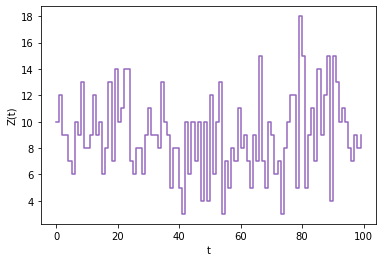
Suppose that $\gamma = 5$, $\nu = 0.5$ and $Z(0)=10$. To simulate a trajectory:

obs_times = [t for t in range(25)]
pop_sizes = bd.simulate.discrete([5, 0.5], model='custom', z0=10, times=obs_times,
                                 b_rate=custom_b_rate, d_rate=custom_d_rate, seed=2021)

The trajectory can be plotted using Matplotlib:

import matplotlib.pyplot as plt

plt.step(obs_times, pop_sizes, 'r', where='post', color='tab:purple')
plt.ylabel('Z(t)')
plt.xlabel('t')
plt.show()

For example:

The parameters can then be estimated from the simulated sample path:

p_bounds = [[0,10], [0,10]]
est = bd.estimate(obs_times, pop_sizes, [1, 1], p_bounds, model='custom',
                  b_rate=custom_b_rate, d_rate=custom_d_rate)
print(est.p)

Which displays the estimate:

[7.029076385718105, 0.6961996442136139]

Model label	\(\lambda_z(\boldsymbol\theta)\)	\(\mu_z(\boldsymbol\theta)\)	\(\boldsymbol\theta\)
`'linear'`	\(\gamma z\)	\(\nu z\)	\(\gamma\), \(\nu\)
`'linear-migration'`	\(\gamma z + \alpha\)	\(\nu z\)	\(\gamma\), \(\nu\), \(\alpha\)
`'pure-birth'`	\(\gamma z\)	\(0\)	\(\gamma\)
`'pure-death'`	\(0\)	\(\nu z\)	\(\nu\)
`'Poisson`	\(\gamma\)	\(0\)	\(\gamma\)
`'Verhulst'`	\(\gamma\left(1-\alpha z\right) z\)	\(\nu\left(1+\beta z\right)z\)	\(\gamma\), \(\nu\), \(\alpha\), \(\beta\)
`'Ricker'`	\(\gamma z \exp\left(-(\alpha z)^c \right)\)	\(\nu z\)	\(\gamma\), \(\nu\), \(\alpha\), \(c\)
`'Hassell'`	\(\frac{\gamma z}{(1+\alpha z)^c}\)	\(\nu z\)	\(\gamma\), \(\nu\), \(\alpha\), \(c\)
`'MS-S`	\(\frac{\gamma z}{1+ \left(\alpha z\right)^c}\)	\(\nu z\)	\(\gamma\), \(\nu\), \(\alpha\), \(c\)
`'Moran'`	\(\frac{N-z}{N}\left(\alpha\frac{z}{N}(1-u) + \beta\frac{N-z}{N}v\right)\)	\(\frac{z}{N}\left(\beta\frac{N-z}{N}(1-v) +\alpha\frac{z}{N}u\right)\)	\(\alpha\), \(\beta\), \(u\), \(\nu\), \(N\)
`'M/M/1'`	\(\gamma\)	\(\nu I_{\{z > 0\}}\)	\(\gamma\), \(\nu\)
`'M/M/inf'`	\(\gamma\)	\(\nu z\)	\(\gamma\), \(\nu\)
`'loss-system'`	\(\gamma I_{\{z < c\}}\)	\(\nu z\)	\(\gamma\), \(\nu\), \(c\)